RUSSIAN ACADEMY OF SCIENCES

INSTITUTE FOR INFORMATION TRANSMISSION PROBLEMS

(KHARKEVICH INSTITUTE)

analytical web gis

GeoTime

Version 2.0

USER GUIDE

Moscow

2008

Summary

The network GIS GeoTime 2.0 is intended for an interactive presentation, analysis and modeling of vector and grid-based geographic information on spatio-temporal processes, which are described by the models with local interaction. Characteristics of such processes vary under influence of the direct topological or functional relations between components of the spatial structure. These components are, in particular, the geographic objects or the neighboring elements of the regular coordinate grid. There are many natural and technogenic processes correspond to the model, such as seismotectonic interactions, dissemination of water effluent of the pollutions in the environment, preparation of the natural catastrophes, as well as social-economic processes.

The system is realized as Java-application. To launch GIS GeoTime 2.0 it is necessary that a virtual Java machine (the version not less then 1.6) has been installed on the user’s PC. GIS loading occurs under Java Web Start technology.

Project leader: Valeri GITIS, Dr.Sci.,

Institute for Information Transmission Problems RAS (Kharkevich institute),

Section of Geoinformation Technologies and Systems
B. Karetnyi Lane 19, 127994 Moscow, GSP-4, Russia, Phone:+7-495-6995096, Fax: +7-495-6500579,

e-mail: gitis@iitp.ru

CONTENS

1. General information. 4

1.1. Data types. 4

1.2. External formats. 4

1.3. GIS-project metadata. 6

1.4. Architecture. 8

1.5. Network function. 9

2. Operations. 9

2.1. Launch window.. 9

2.3. Map window.. 11

2.4. Window of the geo informational layers. 12

2.5. Window of the layer attributes. 12

2.5.1. The attributes of a grid-based layer visualization. 12

2.5.2. The attributes of 3D and 4D grid-based layer visualization. 14

2.5.4. The control of line layer visualization. 17

2.5.5. The control of coordinate grid visualization. 18

2.6. The panel of the visualization management 18

2.7. The panel of the operation management 18

2.8. File group. 18

2.8.1. The operation File>New Project 18

2.8.2. The operation File>Save Project 18

2.8.3. The operation File>Plugin Management 19

2.8.4. The operation File>Load layer 19

2.8.5. The operation File>Import From Catalogue. 19

2.8.6. The operation File>Import From *.flt List 20

2.8.7. The operation File>Export 20

2.8.8. The operation File>Exit 21

2.9. Transformation group. 21

2.9.1. The operation Transform> Raster Filters. 21

2.9.2. The operation Transform>Raster Combination. 23

2.9.3. The operation Transformation>Illumination Model 24

2.9.4. The operation Transform>Correlation in window.. 25

2.9.5. The operation Transform>Isoline Curvature. 25

2.9.6. The operation Transform>Vector Filters. 26

2.10. Group Seismotectonics. 28

2.10.1. The operation Seismotectonics>Seismic Fields. 28

2.10.2. The operation Seismotectonics>RTL.. 32

2.10.3. The operation Seismotectonics> Anomaly Estimation. 33

2.10.4. The operation Seismotectonics> Prognosis Quality Estimation. 37

Fig. 44. 38

3. Plug-in: Seismic flow temporal analysis (GeoSeries) 41

1. General information

The system is realized as Java-application. To launch GIS GeoTime 2.0 it is necessary that a virtual Java machine (the version 1.6 or more) has been installed on the user’s PC. GIS loading occurs under Java Web Start technology. Application of Java Web Start technology allows to use as important positive aspects of Java Applet technology (primarily it is the convenience to disseminate the actual version of the application via Internet), and the advantage of the running without web browser. The last property allows to exclude negative influence of web browser: in particular, to eliminate the additional restrictions on the amount of memory available for Java application. This is a critical factor accepting in attention the significant volume of the geographic data with which GIS GeoTime 2.0 works.

The version supports the operations with geographic data, given in degree coordinates.

The modules of GIS GeoTime are implemented in plug-in technology. This architecture allows flexibly changing GIS functionality.

Three of the plug-ins, which are the large programme systems, are separated: plug-in of cluster detecting in seismic flow, plug-in of temporary event sequence analysis, and plug-in of surface water flow modeling. Plug-in of temporary event sequence analysis is included in the actual version. Another two plug-ins (Seismic flow clusterization: http://www.geo.iitp.ru/geotime/geotime2_plugin_earthquakes.jar and Water flow modeling: http://www.geo.iitp.ru/geotime/geotime2_plugin_surface_flow.jar) can be loaded into the basic version dynamically.

Application of these plug-ins requires special consultations of developers.

1.1. Data types

GIS GeoTime 2.0 supports the operations with 2D, 3D and 4D vector and grid-based data. Usually (but optional) data are structured in a form of GIS-projects. The Project is a set of semantically homogeneous data on some spatial region. It is comfortable to locate each project in separate catalogue as a set of the files of data and metadata. A special configurational file is used for metadata presentation.

The following data types are supported.

· 2D 3D 4D grid-based data.

· Vector-based data:

o Spatio-temporal marked point fields (for example, earthquake catalogues).

o Time series with geographical localization.

o Geographical points.

o Lines.

o Polygons.

· Metadata

1.2. External formats

Vector data are presented by the SHP format (ESRI). Additionally the text tabular format can be used for the point data (event catalogues, time series and geographic points). In this format each table row relates to a separate object:

Year MM DD Long Lat Class HH Min Sec

1980 1 1 76.450 42.950 7.0 0 30 14.0

1980 1 1 74.010 42.350 6.3 23 7 43.0

1980 1 2 72.760 42.050 7.3 1 31 5.0

1980 1 2 78.200 43.180 7.2 20 11 18.0

1980 1 2 73.900 40.680 7.1 20 24 31.0

1980 1 3 73.450 40.580 8.6 9 30 48.0

1980 1 3 74.980 40.880 9.2 11 22 10.0

………………………….

The external format of 2D and 3D grid-based data is the FLT text format (close analog of ASCII grid format used by ESRI). 3D grid data are presented as a sequence of 2D grid slices. Each 2D or 3D layer is accompanied by the text file of metadata. The FLT file consists of three parts: header, data and a description.

The header presents a line<COL> <ROW> <Xbeg> <Ybeg> <Dx> <Dy> <Intr> <Geog>, which includes 8 parameters separated with blanks: COL is number grid columns, ROW is number grid rows, Xbeg is the coordinate of the left grid column, Ybeg is the coordinate of the upper grid row, Dx is the distance between grid columns, Dy is the distance between grid rows, Intr is the indicator (if Intr=1 then to interpolate the data into screen pixel and if Intr=0, then not to use interpolation, Geog is the indicator of the coordinate type (if Geog=1 then geographic coordinates is used, if Geog=0 then Descartes ones is used, note this version is not support Descartes coordinates).

The numerical values of 2D slices are ordered in the nodes by the grid on-left to the right and are divided from the top to down also by blank or new-line. The unknown values are designated as -32768 or as the symbol ".". Data array is followed by the text comment, which begins with an empty row:

141 158 73.5 44.5 0.05 -0.03503185000000001 1 1

4513.0 4513.0 4513.0 4513.0 4513.0 4513.0 4513.0 4513.0 4513.0 4513.0 4513.0 4513.0 4513.0 4513.0 4513.0 4513.0 4513.0 4513.0 4513.0 4513.0 4513.0 4513.0 4513.0 4513.0 4513.0 4513.0 4513.0 4513.0 4513.0 4512.0 4512.0 4512.0 4511.0 4510.0 4509.0 4507.0 4505.0 4503.0 4501.0 4498.0 4495.0 4492.0 4488.0 4484.0 4479.0 4474.0 4469.0 4464.0 4459.0 4454.0 4448.0 4442.0 4437.0 4431.0 4426.0 4420.0 4415.0 4410.0 4404.0 4399.0 4394.0 4390.0 4385.0 4381.0 4377.0 4373.0 4370.0 4366.0 4363.0 4360.0 4358.0 4355.0 4353.0 4352.0 4351.0 4350.0 4349.0 4349.0 4349.0 4349.0 4350.0 4352.0 4354.0 4356.0 4359.0 4362.0 4366.0 4370.0 4375.0 4381.0 4387.0 4393.0 4400.0 4408.0 4416.0 4425.0 4434.0 4444.0 4454.0 4464.0 4475.0 4486.0 4497.0 4508.0 4520.0 4531.0 4542.0 4552.0 4562.0 4572.0 4582.0 4591.0 4599.0 4607.0 4615.0 4622.0 4628.0 4634.0 4639.0 4644.0 4648.0 4652.0 4655.0 4658.0 4661.0 4663.0 4665.0 4667.0 4669.0 4670.0 4672.0 4673.0 4673.0 4674.0 4675.0 4675.0 4675.0 4676.0 4676.0 4676.0 4676.0

…………………………………………………………………………………………………………………………...

……………….. 4593.0 4592.0 4592.0 4591.0 4591.0 4591.0 4591.0 4591.0 4591.0 4592.0 4592.0 4592.0 4593.0 4593.0 4593.0 4593.0 4593.0 4593.0 4594.0 4593.0 4593.0 4593.0 4593.0 4593.0 4593.0 4593.0 4593.0 4593.0 4593.0

Velocities m/sec, H=-110km. Tomography estimates made by IPE RAS G.Kosarev, L.Vinnik et al.

Data processing made by IITP RAS: Interpolation from 39 points: Rmax=700km, Npoints=39, Power=5 and moving averaging with R=30km

2D grid-based data file is attended by a metadata ASCII file, which consists of two rows. The first row contains an optional text, the second one consists a filename of the 2D grids-based layer in *.FLT format.

An example of metadata file for 2D grid-based layer in ASCII format:

1 2 3 4

EuroTopo30.flt

FLT files log in subdirectory with the fixed name DATA.

ASCII format of 3D grid-based data consists of N files that are a sequence of 2D grids-based slices in *.FLT format. Metadata file XXX.XXX consists of N+1 rows. The first row contains the optional text (e.g., boundaries of an interval and a step on Z or T scale), the next rows specify the filenames of 2D grids-based slices in order over the values of Z or T scales.

An example of metadata file for 3D grid-based layer in ASCII format:

1 2 3 4

TOMO-0_M.flt

TOMO10_M.flt

TOMO20_M.flt

TOMO30_M.flt

TOMO40_M.flt

TOMO50_M.flt

TOMO60_M.flt

TOMO70_M.flt

TOMO80_M.flt

TOMO90_M.flt

TOMO100_.flt

TOM110_M.flt

TOMO120_.flt

TOMO130_.flt

TOMO140_.flt

TOMO150_.flt

TOMO160_.flt

TOMO170_.flt

TOMO180_.flt

TOMO190_.flt

TOM200_M.flt

FLT files log in subdirectory with the fixed name DATA.

1.3. GIS-project metadata

GIS-project metadata are of the form XML files. There are three types of XML files: GIS-project file, grid-based layer file и vector-based layer file.

GIS-project file

<name>Central Asia</name>

<file>http://www.geo.iitp.ru/geotime/asia/Asia.gp3</file>

</layer>

<font style="1" size="10">SansSerif</font>

</layer>

</layers>

<gui_config>

</projections>

</gui_config>

</project>

The element project is project basic element of the data description. It contains a sub element layers, in which there is a list of the layers of a given project. The element layer defines each GIS layer. There is the attribute type, which determines the type of the layer: map indicates grid-based layer, vector indicates vector layer, and grid indicates coordinate grid layer.

Grid-based data are loaded from gp3 files (GeoTime grid-based data format) and flt files (external ASCII GeoTime grid-based data format). The type of the file is declared in the attribute source: if the file type is gp3, then source=”archive”, if the file type is flt, then source=”flt”.

The attribute visible=”true” or “false” is declared subject to show or not the layer after the Project loading. The element name declares the name of the layer, the element file declares the name of the corresponding file.

Vector layer can be loaded only from the shp files, and the attribute type is source=”shape”. The attribute visible indicate the same meaning as for grid-based layers. The same touches the elements name and file.

In a description of the spatial coordinates of the coordinate grid for the axes X and Y it is necessary to specify in the degrees the initial coordinate, step of the grid and the ending coordinate. For Z-axis, the same values are specified in meters. For the t-axis, the coordinates and the grid step are specified in milliseconds starting from 0 hours 0 min of 0 sec after 01.01.1970.

The element <gui_config> describes the graphic interface settings. The element <projection> sets two axes of the coordinates, which give a plane of the projection, the directions of the axes and a boundary of the mapped region. If the axis in a plane XY is directed up or to the left then in front of a corresponding figure the sign “-” is placed.
The attribute horizontal corresponds to the ordinate axis and the attribute vertical corresponds to the abscissa axis. The figures correspond to the axes: 1 - axis t, 2 - the axis Z, the 3 - axis the X, 4 - axis Y. The attribute x corresponds to the initial coordinate on the ordinate axis, and the attribute width corresponds to the width of the displayed region. Similarly, the attribute y corresponds to the initial coordinate on the abscissa axes, and the attribute height corresponds to the height of the displayed region.

Grid-based layer file

Example 2:

<root><name>China</name><desc>This layer was created</desc><author>Gitis V.G.</author><x from="72.05" to="131.92340000000002" /><y from="54.9716" to="15.054800000000007" /></root>

project is a main element of the layer description. It includes the subitems name, desc, author, x, y. The subitems x и y fix the layer boundaries: from the attribute “from” till to the attribute “to”.

Vector-based layer file.

Example 3.

config is a main element of the layer description. It includes a set of subitems, which present the attributes of visualization:

color – fix the filling color

border_color – fix the boundary color

scale_attr – the scale attribute (0 by default)

max_value – maximal threshold for point representation (the points with the values more then max_value are not displayed)

min_value – minimal threshold for point representation (the points with the values less then min_value are not displayed)

max_size – maximal representation size (the size for displaying of the points with max_value)

min_size – minimal representation size (the size for displaying of the points with min_value)

h_shift – horizontal shift for the point lettering

v_shift – vertical shift for the point lettering

t_min – minimal time-threshold in ms from 1970 for point representation (the points with the dates less then t_min are not displayed)

t_max – maximal time-threshold in ms from 1970 for point representation (the points with the dates more then t_max are not displayed)

1.4. Architecture

GIS GeoTime 2.0 consists of three subsystems: data storage, data processing and data visualization (Fig. 1).

Fig.1

The data storage subsystem supports dynamical loading and saving data and plug-in. It is divided into four parts: initial and computed GI, plug-in instances, processor of GIS-project compiling, and processor of GIS-project saving. The visualization subsystem support interactive cartographical exploration of GI. The data processing subsystem allows executing of the operations of complex data analysis.

1.5. Network function

GIS GeoTime 2.0 supports integration of data and plug-in which can be distributed on the network servers and the user's computer.

The following network functions are supported:

· Distributed GIS-projects: the possibility of reading GIS-the projects located on the network servers and on the user's computer.

· Distributed GIS-data: the possibility of reading the data located on the network servers and on the user's computer and compiling the GIS-project.

· Distributed plug-ins: the possibility of dynamic plugging of Java modules, located on the network servers and on the user's computer.

· GIS-project saving: saving of the data and metadata on the user's computer.

The diagram of network interaction between the components of the system is shown on Fig. 2. The Web-server with the GIS GeoTime 2.0 core, Web-servers with GIS-projects, plag-ins, data are present on network. The prepared individual user’s GIS-projects, plag-ins and the data can be arranged on the user's computer.

Fig. 2.

The HTML-document that can be run either from the Web-server or from the user's computer is necessary for initialization. The HTML-document contains URL of the GIS GeoTime 2.0 core (the JNLP-file in which specified URL of the configurational XML-file with metadata of the executed GIS-project)

2. Operations

2.1. Launch window

The address of GIS-project window is http://www.geo.iitp.ru/geotime/index.htm. The menu of the launch window is shown on a Fig. 3. The menu consists of the list in which a user can select maximum amount of memory available for the application (from 512Mb till 1500Mb is possible), specify the GIS-projects and plug-ins if it is necessary. First of all a user ought to select amount of memory. After that choosing Start keys it is possible to launch a system with any of the prepared GIS-projects. Then in case of necessity, it is possible to load the plug-in.

(Beta version)

exploits Java Web Start technology

requires JRE 1.6 to be installed

GIS GeoTime II is a comprehensive computer environment for intelligent research of spatio-temporal processes.

USER GUIDE (in Russian, in English)

GIS-projects are loaded with GeoTime II core. It is possible to add plugins using GeoTime II interface: open menu Plugins, run Plugin management and add in the bellow row of the dialog box full pass to the plugin jar-file. There are following plugins at the server:
1. Seismic flow clusterization:
http://www.geo.iitp.ru/geotime/geotime2_plugin_earthquakes.jar
2. Seismic flow temporal analysis:
http://www.geo.iitp.ru/geotime/geotime2_plugin_geoseries.jar
3. Water flow modeling:
http://www.geo.iitp.ru/geotime/geotime2_plugin_surface_flow.jar

Select maximum amount of memory available for the application:

Central Asia	GIS-project on seismotectonic of Central Asia. The project has been developed in cooperation with the Institute of Physics of the Earth RAS under the Program of Presidium of RAS "Electronic Earth"
China	GIS-project on seismotectonic of China region. The project has been developed in cooperation with The Institute оf Earthquake Science, China Earthquake Administration.
Eurotraverse	GIS-project on seismotectonic of Central Europe. The project was made by the data from CD-ROM "The European Geotraverse Database"
North India	This project was carried out under ILTP cooperation program in cooperation with Wadia Institute of Himalayan Geology, Dehradun and India Meteorological Department, New Delhi.
Central Russia	GIS-project on seismotectonic of Central Russia
Kamchatka	GIS-project has been prepared in collaboration with the Institute of Physics of the Earth RAS under the Program of Presidium of RAS "Electronic Earth" and project RFBR 06-07-89139
Ruza District	GIS-project for water surface-flow research
Dmitrov District	GIS-project for water surface-flow research

Fig. 3.

2.2. GIS-project window

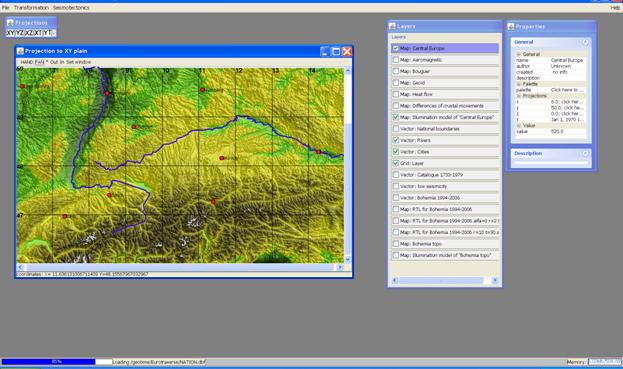
Fig. 4.

GIS-project window contains the map window (at the center), the window of the geo informational layers (to the right), the window of the layer attributes (the extreme on right), the control panel of the visualization (the pop-up panel at the top), the control panel of the operations (the upper panel). Below on the left there is the indicator of the informational resource loading, below on right is the indicator of the random access memory, “Memory” in which, there are two numbers: the first number is amount of the used memory (on the Fig. 4 it is equal 407Mb), the second number is the maximum volume of the allocated memory (on the Fig. 4 it is equal 1016Mb).

The user can change the window disposition and size. It however is necessary to remember that in pressing Alt+F4 the basic window will close

2.3. Map window

Map size changing. It is possible with simple changing of the map window size. The map will vary according to the window (in the given version the map proportion conservation s is not supported). In order to change a map size within the fixed window size a user ought to put the button <Set window> in the window of corresponding map projection. After that, it is necessary to install the map sizes in two coordinates XY (or XZ, YZ, XT, YT, ZT) and to press the button “OK”. If GIS-project is loaded from user PC then the map size is saved automatically after exit the program. The map size can be adjusted with the help of editing XML-file of the project.

Map scale changing. It can be done in two steps: click the button PAN and draw a rectangular area at the map window. Click the button «*» to come back to the initial scale. Click the buttons IN or OUT to increase or to decrease a map scale correspondently.

Map position changing. It is possible to move the increased image of a fragment of the map with the help of a cursor. Click the button HAND, deliver the courses inside the map window, press LMB, and drag the map in necessary direction.

Measurement of the cursor coordinate and reading the active layer values. The cursor coordinates are typed in the window status line. If a grid-based layer is activated (see item 2.4) then corresponding value of the layer appears within the window of the layer attributes.

2.4. Window of the geo informational layers

The window presents the list of Layers, including initial and calculated layers of the GIS-project. The order of the visualized layers on a map is defined by the sequence of the layers in a list: the first layers of the list correspond to the bottom layers of the map

Layer choice. Click the button on the left of the layer name to add a layer in the Layers list. Click the button for a second time to eliminate the layer.

Layer activation. Click LMB on the layer’s name for layer activation. Active layer may not relate the layers, which are chosen for a mapping in the layer list.

Change of the layer order. Click LMB on the layer’s name and drag a cursor to a new position.

2.5. Window of the layer attributes

The window of the layer attributes is intended for a management of cartographical presentation of the layers. At first, it is necessary to activate required layer.

2.5.1. The attributes of a grid-based layer visualization

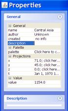There are several categories of the grid-based layer visual attributes (Fig. 5): General, Palette, Projections, Value, and Description.

The category named General includes the following attributes:

1) Bookmark name is a title of the layer;

2) Bookmark author is the name of the layer’s author;

3) Bookmark created is the date and the time of the layer creation.

The values of these attributes are loaded from a layer metadata file and saved in creation and conservation of new layer.

Palette category contains the sole attribute palette. Click a button "change….” to change palette attribute. The window of installation of the of grid-based layer visual parameters appears after that (Fig. 6).

Fig. 5.

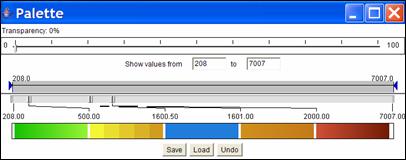
Fig. 6.

On the first line moving a slider, it is possible to set transparency of the grid-based layer.

On the second line moving delimiters or putting the values into the panels Show values from … to …. it is possible to choose the range of the visible part of grid-based layer. Putting LMB on the bellow part of the line, it is possible to divide the grid values into a set of segments.

The third line controls painting of the grid-based layer segments. Click LMB on the left and right sides of the color segments to initialize a window Select color (Fig. 7). Colors inside the segment are interpolated between colors on its boundaries in the scales RGB, HSB or RHSB. In pulling through of a cursor with pressed LKM from one to other boundary of the segment, all its values get the same color.

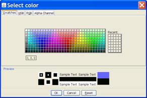
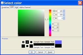
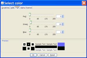
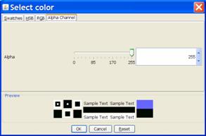
Fig 7.

In the window Select color, it is possible to select color and transparency for the corresponding segment boundary. The transparency varies in the segment by the same way as anther components of color: Alpha is a coefficient of transparency, the value the 0 on scale of transparency corresponds to full transparency, and the value 255 corresponds to non-transparency.

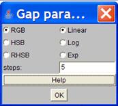After clicking LMB on the middle of the color segment, the window of filling parameters appears (Fig. 8). The left part of the window contains the buttons RGB, HSB, RHSB to select a scale of colors. The right part of the window contains the buttons to select a scale of grid-based values: linear (Linear), logarithmic (Log) and exponential (Exp). Below, the field Steps allow to set up the number of segment color ranges.

Fig. 8.

The Window of installation of the value of the color segment boundary (Fig. 9) appears in pressing LMB.

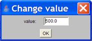
Fig. 9.

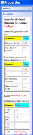
In the bottom, part of the window there is the Description panel, which presents the description of layer. It supports HTML and is kept in metadata of the layer. An example of a description for the layer with estimation of the minimal representative magnitude of earthquakes is shown on Fig. 10

Fig.10.

2.5.2. The attributes of 3D and 4D grid-based layer visualization

In the entity Projections of the window of the grid-based layer attributes (Fig. 5), the values of the layer’s slice are presented. For example, in change of the coordinate of Z (depth) or T (time) the projection XY will be animated. In order to change the slices it is necessary to select an axis and press a key “change…”. A dialog window with the interface to control 3D grid-based layer visualization appears (Fig. 11).

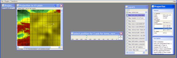
Fig. 11.

Visualization of spatio-temporal 3D grid-based layers presents animated image. Visualization is possible for the slices in three planes: XY (the longitude-latitude plane, time changes with a step according to the grid of the time scale), XT (the longitude-time plane, the latitude changes with a step according to the grid of the latitude scale) and YT (the latitude-time scale, the longitude changes with a step according to the grid of the longitude scale). The choice of the plane is made by pressing of a corresponding button on the control panel of visualization. Three control modes of animated visualization are possible: (1) to run the animation in automatic mode by pressing the button « > », (2) to drag a scale slider, (3) to put the cursor on the left or the right of the slider and to click the key «↑» or «↓».

The button Export starts saving of animated visualized image in GIF-file. The export dialog window is presented on Fig. 12.

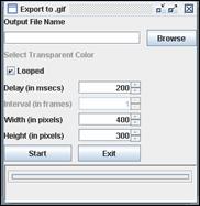
Fig.12.

The control of spatial 3D grid-based layer visualization is analogous. In order to select grid-based layer slices the buttons XY, XZ and YZ are used instead of the buttons XY, XT, YT.

Visualization of 4D grid-based layer allows, fixing the value in the coordinate X, Y, Z, or T to select 3D slice and further choose 2D slices XY, XT, YT XY, XZ, YZ.

2.5.3. The control of point layer visualization

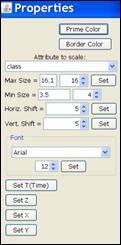
For point layer visualization the circular pictogram is used. There is an interface to choose and control parameters of visualization in a window Properties (Fig. 13). Bookmark Attribute to scale allows to choose the mapped attribute. The parameters of attribute visualization are Prime Color, Border Color, and the size of the pictogram, depended on the attribute value. Bookmarks Max Size и Min Size control the point sizes. The bookmarks have to fields. The first field determines maximal (minimal) value of the attribute; the second field determines corresponding size in screen pixels. Bookmarks Horiz. Shift and Vert Shift determine a shift of the upper left corner of a caption regarding the center of the pictogram in screen pixels. Bookmark Font determine a font type and size. The parameters are mapped by the buttons Set.

Fig. 13.

Four buttons in the bottom part of the window Properties activate the control of visualization over the axes of T, Z, X, Y (if specified in catalogue the number of attributes less than four, then the corresponding buttons are absent).

Let us consider the operations of visual research of the event of catalogues.

The catalogues are presented by Shp-files (or they could be convert in Shp-files using the plug-in Import from Catalogue). In addition to Shp-files can be presented by dbf- and xml-files, containing the attributes as well as for each of the events (time of event, value, name etc) as information about visualization of the point layer integrally. Each event can content three spatial coordinates X, Y, Z, and a temporal coordinate T, the value of event is an optional numeric attribute except X, Y, Z, T. The text is mapped on the screen if the attribute “Text” is filled.

The following operations of visual research are supported.

1. Representation of the catalogues in coordinates XY, XZ, YZ, XT, YT, ZT.

2. Launching of the animated is presentation of the catalogue over any of the coordinates except the coordinates relating to the projection plane. For one of these coordinates it is possible to define the interval of scanning, and over other coordinate to implement the animated mapping.

For example, it is possible to choose a projection XY, tan interval (Z₁, Z₂) for axis Z, and to present animated mapping over T coordinate. Let us denote this operation as XY(t|z(Z₁,Z₂)). Then operation XZ(y|t(T₁,T₂)) means, that events in the interval (T₁,T₂) are represented in projection XZ for animated mapping over the y coordinate.

The button Set T (Time) starts the slider of animated visualization of a point layer in time (Fig. 14).

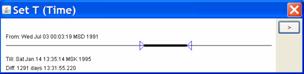
Fig. 14.

The sliders Set X, Set Y и Set Z are similar to the slider Set T (Time). It is possible to define the interval, which selects a subset of mapped events. Then it is possible to put the cursor within the interval and draw the interval by the cursor. Click the button “>”to move the interval automatically with a step equal to 0.01 of the data range along the corresponding axis. Click the button “||”to stop the intervalдля остановки надо прожать кнопку.

An example of visualization of the Kamchatka earthquake catalogue from 1962 till 2004 is shown at Fig. 15 (http://www.geo.iitp.ru/geotime/kam4atka.html). The earthquake epicenters with the depth from 50 to 100km are shown at Fig 16. The window Set Z is shown on the upper part of the Figure. This operation presents animatedly the variation of the epicenters in the plane XY when the interval shifts from the depth 0 to the depth 652km. It is possible to conclude that the increasing the depth leads the strip of epicenters to North-West direction. The earthquake epicenter XY and XZ projections with latitudes from 50º to 52 º are shown at Fig. 17.

Fig. 15.

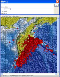
Fig. 16.

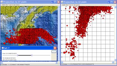
Fig. 17.

2.5.4. The control of line layer visualization

The window of the linear layer attributes coincides with the window of the point layer attributes (Fig. 14). The bookmark Config initializes the dialog window with interface for selection of line prime color and thickness (Fig. 18)

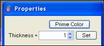
Fig. 18.

2.5.5. The control of coordinate grid visualization

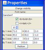The coordinate grid visualization window is represented at Fig. 19. The following parameters are optional for coordinate grid visualization: grid visibility, font parameters, grid intervals and grid step (the interval is equal to the number of temporary slices is recommended to use for the axis T). Click the button Redraw to map the parameters.

Fig. 19.

2.6. The panel of the visualization management

The panel of the visualization management (Fig. 20) realizes a choose of the visualized plane (the buttons XY, XT, YT XY, XZ, YZ). Click the button in order to map the corresponding cartography window. Second click removes the window.

Fig. 20.

2.7. The panel of the operation management

The panel of the visualization management opens three bookmarks File, Transformation, and Seismotectonics, which includes the following groups of operations (Fig. 21).

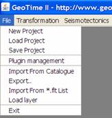
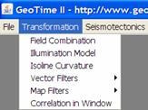
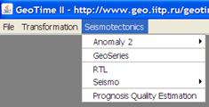
Fig. 21.

2.8. File group

File operations are New Project, Load Project, Save Project, Plug-in management, Import From Catalogue, Export, Import from *.flt List, Load layer, Exit.

2.8.1. The operation File>New Project

The operation New Project completes the project execution, empties memory for a new project. The button New Project opens the window Save Project? to select the option to save or not to save current project. For the option Save the window Select filename for project XML appears to select saved information.

2.8.2. The operation File>Save Project

The operation Save Project opens the window Select filename for project XML to select saved information.

2.8.3. The operation File>Plugin Management

The operation Plugin Management opens the window (Fig.22) in which a user inputs the address of the loaded plug-in.

Fig. 22

2.8.4. The operation File>Load layer

The operation Load layer opens the window (Fig. 23) for selection of a layer. After the layer is selected then it is necessary to press the button Open.

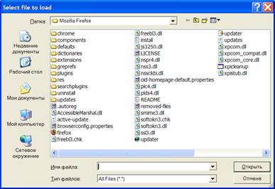
Fig.23.

2.8.5. The operation File>Import From Catalogue

The operation supports import of the event catalogue in ASCII format. The catalogue (e.g., earthquake catalogue) is a sequence of events ordered in time. Any event is presented by the row in which the coordinates X, Y, Z, T, values of event, accuracy of measurements etc. are given. Spatial coordinates are given by decimal digits and time is given as year, month, day, hour, minute, second. The delimiters are spaces or line feeds. The header can be at the first line. The first line of the catalogue must be open without a space. There is no an empty row at the end of the ASCII file.

The dialog window of the operation (Fig. 24) uses a standard interface.

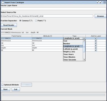
Fig. 24.

2.8.6. The operation File>Import From *.flt List

The option supports import 2D and 3D grid-based layers from ASCII to format FLT.

Dialog window Import from FLT (Fig. 25) contains a standard interface to browse metadata and import a grid-based layer file.

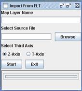
Fig. 25

2.8.7. The operation File>Export

The option supports export 2D grid-based layers from GP3 to FLT format as well as export of vector-based layers in SHP format. Dialog window Export (Fig. 26) contains a standard interface.

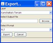
Fig. 26.

2.8.8. The operation File>Exit

The option Exit closes a GIS-project.

2.9. Transformation group

Group Transformation includes a set of general analytical transformations: Field Combinations, Illumination Model, Isoline Curvature, Vector Filters, Raster Filters, Correlation in Window.

2.9.1. The operation Transform> Raster Filters

Operations of 2D, 3D and 4D grid-based layer filtering are executed for all 2D grid-based slices of user-defined plane XY, XT, YT XY, XZ, or YZ. A rectangle-moving window is used in operations mean, median, RMS, local anomalies, maximum, minimum, maximum-minimum. Spatial sizes of the window are km. The values of the adjacent grid notes are used in operations gradient module и gradient azimuth.

The dialogue window of the option contains a standard interface (Fig. 27). There are panels to select a layer to be processed by the name (Select Layer To Process), type of transformation (Select Filter), a plane of thansformation (Select Projection, buttons X axis, Y axis, Z axis, T axis), sizes of the moving window (Defined window size, buttons X size (km), Y size (km), Z size (km), T size), and the output layer name (Output Layer Name).

The button <Preview> is to look preliminary the result, the button <OK> is to save the result, the button <Cancel> to exit of operation.

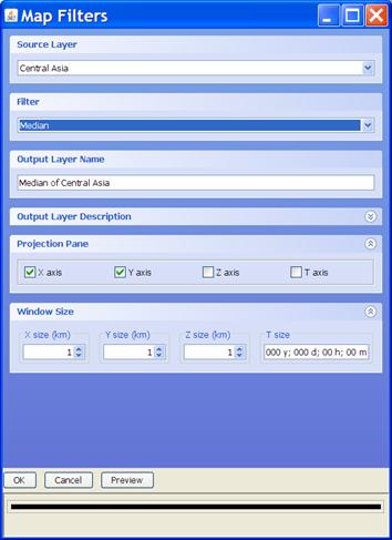
Рис. 27.

Mean is averaging. Output value y_j at a grid point j is equal to average of the input grid values x_i within moving square window with size 2R in km.

where summation is made for all grid cells which are crossed with moving window, is a size of a part of the cell (with the grid knot i), which is covered by j moving window, x_i – value in grid knot i.

Median is median smoothing. Output value y_j at a grid point j is equal to median of the input grid values x_i within moving square window with size 2R in km.

RMS is calculating the grid layer of standard deviations. Output value RMS_j at a grid point j is equal to standard deviation of the input grid values x_i within moving square window with size 2R .

RMS_j

Local anomalies is trend removing. Output value Local anomalies_j at a grid point j is equal to standard deviation of the input grid values x_i within moving square window with size 2R.

Gradient module is calculating the absolute value of the gradient.

Gradient module(i)=(A²+B²)^1/2

where

	i4
i1	I	i2
	i3

A=(x_i2 -x_i1 )/(i2 -i1 ), B=(x_i4 -x_i3 )/(i4 -i3 ),

(i2 -i1 ) and (i4 -i3 ) are distances between grid knots (i2 and i1 ) and (i4 and i3 ) in km.

Gradient azimuth is calculating the azimuth of the gradient:

Azimuth(i)=A/B, where, where the notations are giver before.

Maximum is selection of maximal value within moving window. Output value Maximum_j at a grid point j is equal to maximal value of the input grid values x_i within moving square window with size 2R.

Minimum is selection of minimal value within moving window. Output value Minimum_j at a grid point j is equal to minimal value of the input grid values x_i within moving square window with size 2R.

Maximum - Minimum: is calculating difference between Maximum and Minimum. Output value (Maximum – Minimum)_j at a grid point j is equal to (maximal value -minimal value) of the input grid values x_i within moving square window with size 2R.

2.9.2. The operation Transform>Raster Combination

The option supports calculating the 2D, 3D and 4D grid based layer with the help of user-defined function of another grid layers with use elementary functions, logical and algebraic operations. The arguments are the identifiers of the grid layers. On calculations, all grid layers selected as arguments and output grid-based layer are reduced automatically to the uniform grid. On default, a grid step is defined equal to a minimal step of the grid layers involved in operation. The dialog window contains a standard interface (fig. 28).

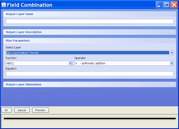
Fig. 28

The list of GeoTime elementary functions is given bellow:

Elementary functions
ABS()	Absolute value of grid layer data (grid layer descriptor is in the parenthesis)
ATAN()	Arctangent of grid layer data (grid layer descriptor is in the parenthesis)
BLK()	BLK(x)=1, if x is defined, BLK(x)=0 otherwise (grid layer descriptor is in the parenthesis)
COS()	Cosine of grid layer data (grid layer descriptor is in the parenthesis)
DAY(year, month, day)	Number of days from 1970.01.01
EXP()	Exponent of grid layer data (grid layer descriptor is in the parenthesis)
IF(a, b, c)	If logical expression a is true, then the result is b , c in otherwise. E.g., expression IF($1>0,$1-$2, -32767) means, that if the values of the grid layer $1>0, then a new grid layer values are equal to differences between the values of the grid layers $1 and $2, else the result is -32767 (dummy value)
INTR(x, x₁, y₁, [,x₂, y₂,...])	Values of the layer defined as peace-wise function, which is given by the notes (x_i, y_i). E.g., expression INTR($1,20,-30,37,99,41,-50): Grid layer values $1 are the arguments, if the value <20 then the result value is -30, if values from 20 till 37 then output values increase linearly from -30 till 99, if values from 37 till 41 then output values decrease linearly from 41 till -50, if values >41 then the result value is -50.
LN()	Natural logarithm of grid layer data (grid layer descriptor is in the parenthesis)
LG()	Decimal logarithm of grid layer data (grid layer descriptor is in the parenthesis)
MAX(,)	Maximum of grid layer values (grid layer descriptors are in the parenthesis)
MIN(,)	Minimum of grid layer data (grid layer descriptors are in the parenthesis)
RAND()	Result is the value of input grid layer plus random noise (grid layer descriptor is in the parenthesis)
ROUND()	Round-up of grid layer data (grid layer descriptor is in the parenthesis)
SIN()	Sinus of grid layer data (grid layer descriptor is in the parenthesis)
SQRT()	Square root of grid layer data (grid layer descriptor is in the parenthesis)

2.9.3. The operation Transformation>Illumination Model

The illumination model of the grid-based layer is presented at Fig. 4. There are three parameters in the dialog window (Fig. 42): Azimuth is the angle between the light source and North, Angle is the angle between the light source and horizon, Vertical factor is a factor by which the grid-based values layer are multiplied, Refinement factor is a factor of decreasing step of the grid, which enhances the image quality.

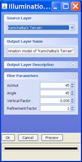
Fig. 29.

2.9.4. The operation Transform>Correlation in window

The option supports calculation of the 2D, 3D or 4D grid-based layer, the values of which are equal to correlation coefficients of two grid layers estimated within 2D, 3D or 4D moving window correspondently (Fig. 30) The layers are interpolated automatically a uniform coordinate grid. By default, the step of the uniform grid gets out to equal minimal grid step of used layers. Transformation of layers to more detailed grid is carried out by means of bilinear interpolation.

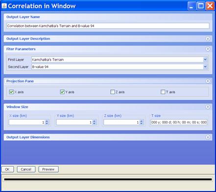
Fig. 30.

2.9.5. The operation Transform>Isoline Curvature

The option calculates a curvature of the grid-based layer isolines according to the following expression:

Where is a plane point, the value of grid-based layer at the point . The dialogue window is presented at Fig. 31. The model of the map of the curvatures of the Earth surface isolines of Kamchatka region is presented at the Fig. 32: red color shows ridges, blue color shows thalwegs (valley-line).

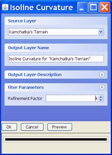
Fig. 31.

Fig. 32.

2.9.6. The operation Transform>Vector Filters

The option supports two types of transformations from line and point layers to 2D grid-based layers: Distance from Vector objects and Closeness to Vector objects. Distance measure in coordinates XY is km, in T is days. The dialogue window is presented at Fig. 33:

Max R (km) and ΔT (days) are filter Parameters

are the buttons for closing or opening the bookmark.

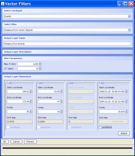
Fig. 33.

Distance from Vector objects is calculation of 2D or 3D grid-based layer of the distances between the grid knots to the nearest point of vector layer. If the input vector layer is 2D layer, then the output grid-based layer dimension will be 2D. If the input vector layer is 3D layer, then the output grid-based layer dimension will be 3D layer. E.g., input layer is a catalogue in coordinates XYT. If parameters for the coordinates XYT are defined then the output layer dimension will be 3D. If flag Undefined is fixed for the axis T then the output will be 2D grid-based layer calculated on all points of the catalogue.

The distance from a grid knot i, in coordinates X, Y, to the nearest point n is calculated in Euclid metrics. If flag Undefined is fixed for the axis T then distances are calculated for all points of layer. If flag Undefined is not fixed for the axis T then each spatial slice of 3D grid-based layer is calculated on the points within temporal interval ΔT (days). If there are no points within the user defined window (with parameters R , ΔT) then the distance is determined as R. Closeness to Vector objects is calculation of 2D and 3D grid-based layer of closeness of the grid knots and vector layer. Closeness is defines as .

2.10. Group Seismotectonics

Seismotectonics operations are Anomaly detection (Anomaly 2), GeoSeries, RTL, Seismic fields (Seismo), Prognosis Quality Estimation.

2.10.1. The operation Seismotectonics>Seismic Fields

The operation supports estimation a set of spatio-temporal patterns of the seismic flow parameters (Fig. 34).: minimal representative magnitude (Min Magnitude Estimation), a slope of the graphic repetition (B-value Estimation), and seismic activity (Seismic Activity Estimation)

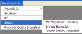
Fig 34.

Two types of estimations are possible. In the first case, it is assumed that Mmin or/and b-value are constants in all spatio-temporal area under study. Therefore, the parameters can be estimated by all earthquake catalogue. In the second case estimation of Mmin, b-value and seismic activity look like 3D grid-based fields and are calculated in everyone of the grid layer points by subcatalogues of events in moving rectangular windows with the user defined sizes ΔX, ΔY, ΔT. For all options the uniform dialogue window is used. It consists of several bookmarks, which can be reduced and be decompressed (Fig. 35):

1. Main window.

2. Window of Output Layer Description.

3. Window of Filter Parameters.

4. Window of the parameters (sizes) of the estimating moving window Window Size.

5. Window of the parameters of calculated grid-based layer Output Layer Dimensions.

6. are the buttons, which are reduce and decompress the dialogue window.

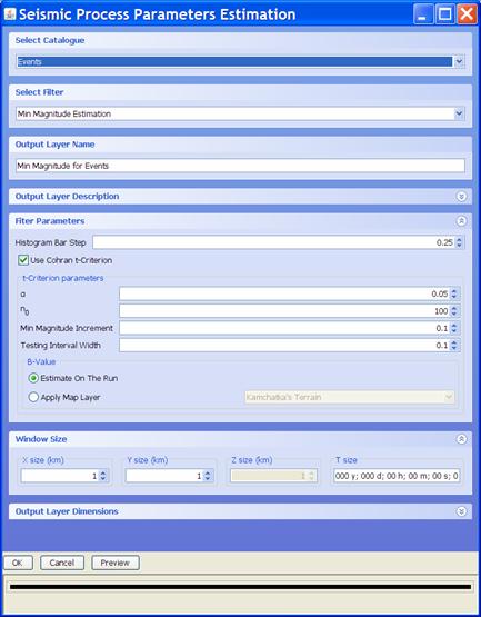
Fig. 35.

The option Min Magnitude Estimation

There are the following operations in the dialogue window:

1. Selection of earthquake catalogue (Select Catalogue)

2. Selection of one of the options: estimation of the minimal representative magnitude of earthquakes (Min Magnitude Estimation), estimation of a slope of the graphic repetition (B-value Estimation), and estimation of seismic activity (Seismic Activity Estimation)

3. Definition of the output layer name.

4. The button “” opens the window of output layer description. The window supports the automatical recording of the parameters of the operation and the possibility of text editing.

The estimation of minimal magnitude of earthquakes (Mmin) starts from definition of the parameters in the window Filter Parameters: definition of the magnitude histogram step (Histogram Bar Step) for estimation of the initial Mmin approximation.

If the flag “Use Cohran t-Criterion” is absent, then this approximation is equal maximum value on the magnitude histogram (if several maximal histogram intervals are the same then the initial Mmax approximation corresponds to the left maximum).

If the flag “Use Cohran t-Criterion” is present”, then t-test is used for Mmin estimation and the following parameters are necessary to define:

1. A significance level α of H₀ Hypothesis, according to which the events in the magnitude interval Testing Interval Width and all the events with more magnitudes belong to one exponential distribution.

2. A normalizing coefficient n₀, which specifies the test sensitivity. The typical values of are n₀=50200.

3. An increment of current value of Mmin after H₀ Hypotheses is rejected.

4. An interval Mmin value (Testing Interval Width) for testing of hypothesis.

Switch “Estimate on the Run”

“Estimate on the Run” option estimates the parameter of exponential distribution (b-value) for each 3D grid point by the events in mowing window, the magnitude of which is more or equal the value of current magnitude under testing. The alternative option Apply Map Layer allows to use b-values from the defined grid-based layer, which is selected of the pulldown list.

The Window Size supports definition of the rectangular parallelepiped, which is use as moving window: Xsize, Ysize, Tsize (Zsize is inaccessible).

The window Output Layer Dimensions supports definition of output grid-based layer.

The option B-value Estimation

The difference in management of b-value estimation from the previous option consists only in contents of the bookmark Filter Parameters (Fig. 36).

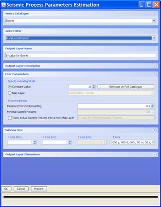
Fig. 36

Switch Specify min Magnitude contains the following two panels:

1. The panel Constant value defines that the value of Mmin will be used for estimation of each value of the b-value grid-based layer. The value of Mmin can be define by user as well as estimated by the whole earthquake catalogue. In the last case the button Estimate on Full open the window of Mmim and b-value estimation by the whole catalogue (Fig. 37).

2. The panel Map Layer defines that the values of Mmin will be taken from the user selected layer.

Trustworthiness

The bookmark Trustworthiness contains the panel Relative Error not Exceeding to define the maximal value of the relative error of b-value estimate, which specifies the minimal necessary sample size of events.

If the button Track Actual Sample Volume is activated then the values of a sample sizes in moving window are traced in a special layer.

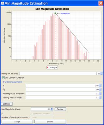
Fig. 37.

There are the following control parameters:

2. A normalizing coefficient n₀, which specifies the test sensitivity. The typical values of are n₀=50200.

3. An increment of current value of Mmin after H₀ Hypothesis is rejected.

4. An interval Mmin value (Testing Interval Width) for testing of hypothesis.

The button Accept is to take the Mmin estimate. After that the Mmin value enter to the main dialogue window (Fig. 36), and the window (Fig. 37) is closed.

The option Seismic activity Estimation

The difference in management of seismic activity estimation from the previous option consists only in contents of the bookmark Filter Parameters (Fig. 38).

Base Magnitude is the value of the magnitude, for which seismic activity is calculated.

Magnitude interval is the interval for seismic activity estimation.

Seismic activity is defined as number of earthquakes in the interval with Base Magnitude in the centre and with the width Magnitude interval normalized on time per 1 year and on area per 1000 km².

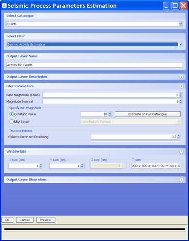
Fig. 38.

2.10.2. The operation Seismotectonics>RTL

The operation RTL supports calculation of the following grid-based layer by an earthquake catalogue (Fig. 39):

Where:

· X,Y,T – the coordinates of 3D grid.

· n – the number of event.

· is the value of event (magnitude or class); only events with are under consideration; are the user defined parameters.

· is earthquake energy; are the user defined parameters.

· α is a degree (e.g., α = 0.33), α is the user defined parameter.

· ε is a user defined threshold.

· r_n [km] is a distant from a grid not to the event.

· t_n [day] is a temporal interval from a grid knot to the event.

· R [km], T [day] are the user defined coefficients of decrements.

· , are the user defined degrees. It is defined on default , .

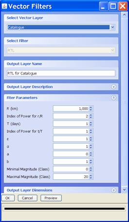
Fig. 39.

2.10.3. The operation Seismotectonics> Anomaly Estimation

The operation Anomaly Estimation supports detection of temporary nonstationarity in spatio-temporal 3D grid-based layer.

The input 3D grid-based layer is a set of time series related to each node of the spatial grid. It is assumed that time series of a parameter of seismic flow is stationary in time. Some of statistical characteristics of the time series change in earthquake preparation. The problem of temporary anomaly detection defines as a problem of comparison of two sample sets relating to two random sample sets. The current observation interval is divided into two consecutive sub-intervals, for which the former one is several times longer than the latter. The duration of both sub-intervals are determined by the researcher depending on the statistical properties of the background signal within the interval without precursor and on the expected duration of anomalous. The problem is reduced to testing the hypothesis of statistical homogeneity of two random sample sets belonged to the sub-intervals. The hypothesis about the coincidence of parameters of the sample set distributions is tested by a certain statistics, which depends on the selected statistical model.

If anomaly is absent, then the values of output, grid-based layer is random variables with the mathematical expectation are 0 and the variance 1. The large positive and negative values are considered as anomalies.

The operation Anomaly Estimation contains several options (Fig. 40): Independent Variates, Independent Variates with block, Markov model, Markov model with block, Dynamic detection, Dynamic detection with block.

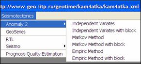
Рис. 40.

The option Independent Variates

It is assumed that the time series at any point of spatial grid of the input 3D layer are described by the random sequence with independent Gauss variables. Let us denote the mathematical expectation of the variables at T₁ and T₂ intervals as and , assume that the variations on both intervals are equal . The dialogue window of the option is at Fig. 41. The option calculates 3D grid-based layer of statistics

Where:

, , , , , , C is a Dispersion estimate Coefficient (Fig. 41), S is a variation of the data over the region within T₂interval.

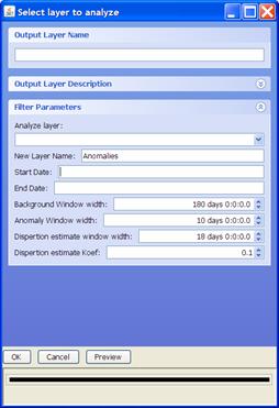
Fig. 41.

Output Layer Name is the panel for the name of output layer.

Output Layer Description is the bookmark for recording the output layer metadata.

Filter Parameters is the bookmark for definition of the parameters.

Analyze layer is a panel for the name of input layer.

New Layer Name is the panel is not use in the version

Start Date, End Date are the panels for definition of the output layer dates.

ackground Window width is the panel dor definition of the 1^st temporal interval duration T₁.

Anomaly Window width is the panel for definition of the 2^nd temporal interval duration T₂ (the interval is comparable with duration of the anomaly).

The option Independent Variates with block

The option allows to eliminate the effect of anomalies on the average value of the 1^st interval. To this effect the time series values, which differ significantly of the average value of the 1^st interval, are skipped of the 1^st window.

The dialogue window (Fig. 42) differs from the previous one by only the row Anomaly level. If statisitics t is more than Anomaly level then the 1^st is locked and the average μ₁ is not change.

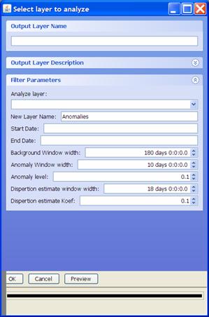
Fig. 42.

The option Markov model

This option differs of the option Independent Variates thereby only independence of the time series samples is not assumed. It is supposed that time series corresponds to Предполагается, что значения ряда соответствуют Markov Gauss linear process. Therefore, another estimation of variation of the difference between averages on T₁ and T₂intervals is used. The dialogue window is the same as for the option Independent Variates.

The option Markov model with block

The option is similar to the option Independent Variates with block.

The option Dynamic detection

At the previous options the statistics was used that is equal the ratio of the difference between averages on T₁ and T₂intervals to the estimation of root-mean-square of this difference. It is possible to apply empiric estimation of the root-mean-square. Let us consider time series and difine 3 sequential and non-overlapping intervals , и . Let us time coincides with the last sample of the interval . Starting from an estimation of the average is known, starting from an estimation of the average is known. After that a standard deviation of is estimated on the interval . Thus by the moment is known the statistics

Where:

The dialogue window Select layer to analyze (Fig. 43) differs from the window of the option Independent Variates by the additional two panels:

The panel Variance estimate window width defines the duration of the interval T₃;

The panel Variance estimates Coef defines the correction of the estimation of standard deviation.

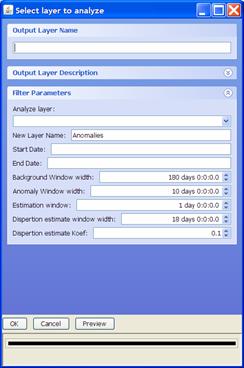
Fig. 43.

The option Dynamic detection with block

The option is similar to the option Independent Variates with block.

2.10.4. The operation Seismotectonics> Prognosis Quality Estimation

This module provides the user with the opportunity to estimate several parameters for a 3D grid-based layer representing anomalies. The anomalies are supposed to exist in every moment (corresponding to each time-slice of input layer) and they are approximated in spatial space by two-dimential Gaussian functions: , where – position vector of an arbitrary point in space, – position vector of seismic center, a – coefficient referred to as relative amplitude, – normalized Gaussian function with center in and variance σ²> 0, so that . The following parameters are estimated for each time-slice:

– location of anomaly center (in XY space)
σ – spread of anomaly (in XY space)
a – anomaly relative amplitude
anomaly absolute amplitude
anomaly energy
anomaly volume
β – anomaly detection certainty, that ranges within closed interval [0..1] and is equal to , where α is the anomaly energy to noise energy ratio.

In order to estimate anomaly parameters, click button [Generate a new Anomaly Time Series Layer] from the main window of Prognosis Quality Estimation plug-in (Fig. 44).

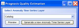
Fig. 44

Then specify input 3D grid-based anomaly layer – Anomaly Map Layer (Fig. 45). Varying parameters from the group “Iterate σ (km)” enables the user to adjust the range (in exponential scale) and iterations count for parameter σ while searching for the most appropriate spread of anomaly. Gaussian Precision denotes the radius of circle in XY space (measured in σ-units) coinsiding with the center of Gaussian function, outside this circle the value of Gaussian function is assumed to be equal to zero in order to simplify computations.

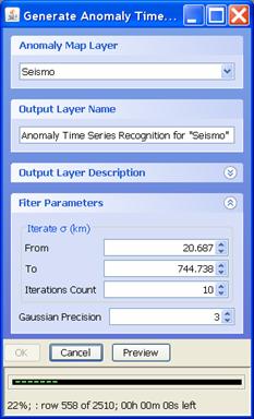
Fig. 45

Once the new vector layer containing anomaly parameters estimations has been generated, one can preview the results exploiting the special graphical tool by selecting in main window the layer to be analyzed and pressing [Preview] button (Fig. 46).

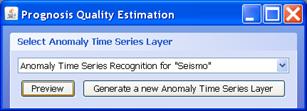
Fig. 46

In Anomaly Time Series Preview frame there are displayed a group of plots for anomaly parameters (Fig. 47). All the plots are bound to the same timeline. It is possible to specify in the panel “Plots to Display” which anomaly parameters should be displayed. “Certainty Threshold” parameter is used to indicate on the timeline the regions with the Certainty excessing the parameter value. Regions filled with green stand for noise. There is a possibility to select any point shown on the plots. In this case, all the parameters relating to this point are displayed in “Selection” panel. Moreover, if the option “Adjust Visible Domain for Vector Layer” is set, the time interval selection slider in “Set T”-control for corresponding vector layer becomes automatically positioned around the selected time value (Fig. 48).

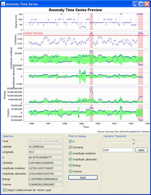
Fig. 47

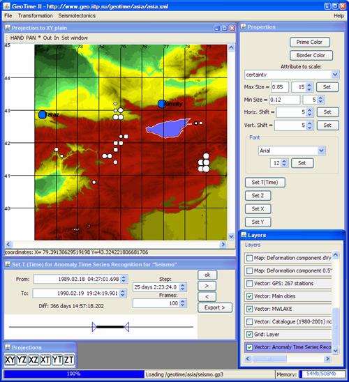
Fig. 48

3. Plug-in: Seismic flow temporal analysis (GeoSeries)

Plug-in downloads all vector layers with points. The dialog window of the plug-in GeoSeries is presented at Fig. 49.

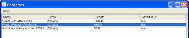
Fig. 49

Column Name contains point layer names, Type is layer type, Length is layer size.

To start analysis it is necessary to select the catalogue: to put the cursor on the name of catalogue and click RMB. The dialogue window, Fig. 50 is open

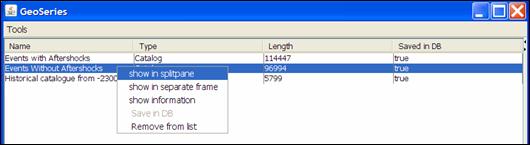
Fig. 50

The panel Show in splitpane is for data visualization in a part of the window.

The panel Show in separate frame is for data visualization in a separate window.

The panel Show information is to show metadata

The panel Remove from list is to erase data from the list.

The result of Show in splitpane operation is presenred at Fig. 51. To control visualization it is necessary to put cursor on the image of the catalogue and to click RMB.

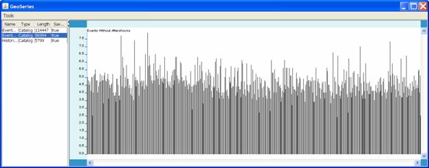
Fig. 51

For activation of the window for visualization management it is necessary to put cursor on the image of the catalogue and click RMB (Fig. 52). The optijns of visualization are clear by their titles.

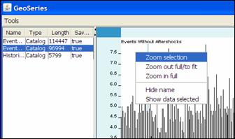
Fig.52

Zoom selection is definition of the interval of visualization (click LMB and drag cursor within the interval, click RMB and to select an option, Fig. 53)

Zoom out full/to fit is to come back to initial presentation of the catalogue.

Zoom in full is to present time series with maximal zoom.

Hide name is to hide the name of the data.

Show data selection is to visualize the time.

Plug-in GeoSeries includes the following set of instruments (Fig. 53):

The panel Flow Density is calculation of the density o epicenters.

The panel Minimum Magnitude is estimation of the minimal representative magnitude.

The panel B-value is estimation of the B-value/

The panel Activity is estimation of the seismic activity.

The panel Histogram is plotting a histogram.

The panel RTL is estimation of RTL

The panel Anomaly detection is a set of tools for anomaly detection:

The panel Independent variates is detection of anomalies for the time series in depended variables.

The panel Markov process is detection of anomalies for the time series in Markov variables

The panel Empirical method – is detection of anomalies by empirical estimation.

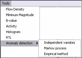
Fig. 53

After selection of the option the window with corresponded name is open (Fig. 54). To open the menu of analytical operations it is secessary to click the panel Option.

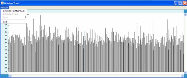
Fig. 54.